Une question?

Notre blog : IA et
vision industrielle
Notre blog : IA et vision industrielle
Articles et actualités de l'équipe Scortex
Articles et actualités de l'équipe Scortex
Catégorie
Catégorie
Tous
Education
Solution
News
Interviews

Comment Saverglass fiabilise l'inspection de ses bouteilles premium grâce à l'IA de Scortex
Equipe Scortex
Défauthèque industrielle : 8 erreurs à éviter lors de sa création
Equipe Scortex

Checklist défauthèque : les 15 points essentiels
Equipe Scortex
Créer une défauthèque industrielle : guide pratique
Equipe Scortex
Comment construire une défauthèque qualité efficace ?
Equipe Scortex

Comment identifier les défauts visuels critiques avant les réclamations client
Equipe Scortex
5 leviers pour améliorer l’analyse qualité
Equipe Scortex

Optimiser la performance qualité tout en réduisant rebuts et retouches
Equipe Scortex

Réduire les coûts cachés grâce au contrôle visuel automatisé

Comment structurer une défauthèque qualité pour sécuriser vos décisions
L'équipe Scortex

Protéger l’image des marques grâce au contrôle qualité des produits de luxe assisté par IA
L'équipe Scortex

Comment sécuriser le contrôle qualité des pièces métalliques avec l’IA
L'équipe Scortex

Automatiser le contrôle qualité des pièces en injection plastique par IA
L'équipe Scortex

Fiabiliser le contrôle qualité packaging avec un contrôle visuel automatisé
L'équipe Scortex

Comment sécuriser le contrôle qualité cosmétique grâce à l'automatisation
L'équipe Scortex

Contrôle qualité cosmétiques et packaging : fiabiliser l’inspection des surfaces exigeantes grâce à l’IA
Equipe Scortex

Contrôle qualité par l'IA : Scortex et IAR Group unissent leurs forces pour transformer le contrôle qualité industriel grâce à l'IA
L'équipe Scortex

7 missions clés d'un Responsable Qualité pour un contrôle qualité optimal
L'équipe Scortex

Comment aller au-delà des machines de tri qualité grâce à l'IA
L'équipe Scortex

Comment optimiser la qualité de production avec l'intelligence artificielle ?
L'équipe Scortex

Qu'est-ce que la traçabilité en contrôle qualité ? Explications simples
L'équipe Scortex

En quoi le contrôle qualité manuel et automatisé sont-ils complémentaires ?
L'équipe Scortex

Interview avec Hugues Poiget, CEO de Scortex
L'équipe Scortex

Dans les coulisses d'une marque de luxe qui a révolutionné le contrôle qualité de ses rouges à lèvres
L'équipe Scortex

Comprendre la norme qualité dans l'industrie automobile
L'équipe Scortex

5 façons de contrôler la qualité d'un produit
L'équipe Scortex

Défauthèque qualité : à quoi ça sert ?
L'équipe Scortex

Production cosmétique : défauts qualité visuels à éviter
L'équipe Scortex

Injection plastique : définition et fonctionnement
L'équipe Scortex

Les applications de l'intelligence artificielle en contrôle qualité
L'équipe Scortex

L'industrie 4.0, qu'est-ce que c'est ? Explications
L'équipe Scortex

Les avantages de l'inspection automatisée en contrôle qualité
L'équipe Scortex
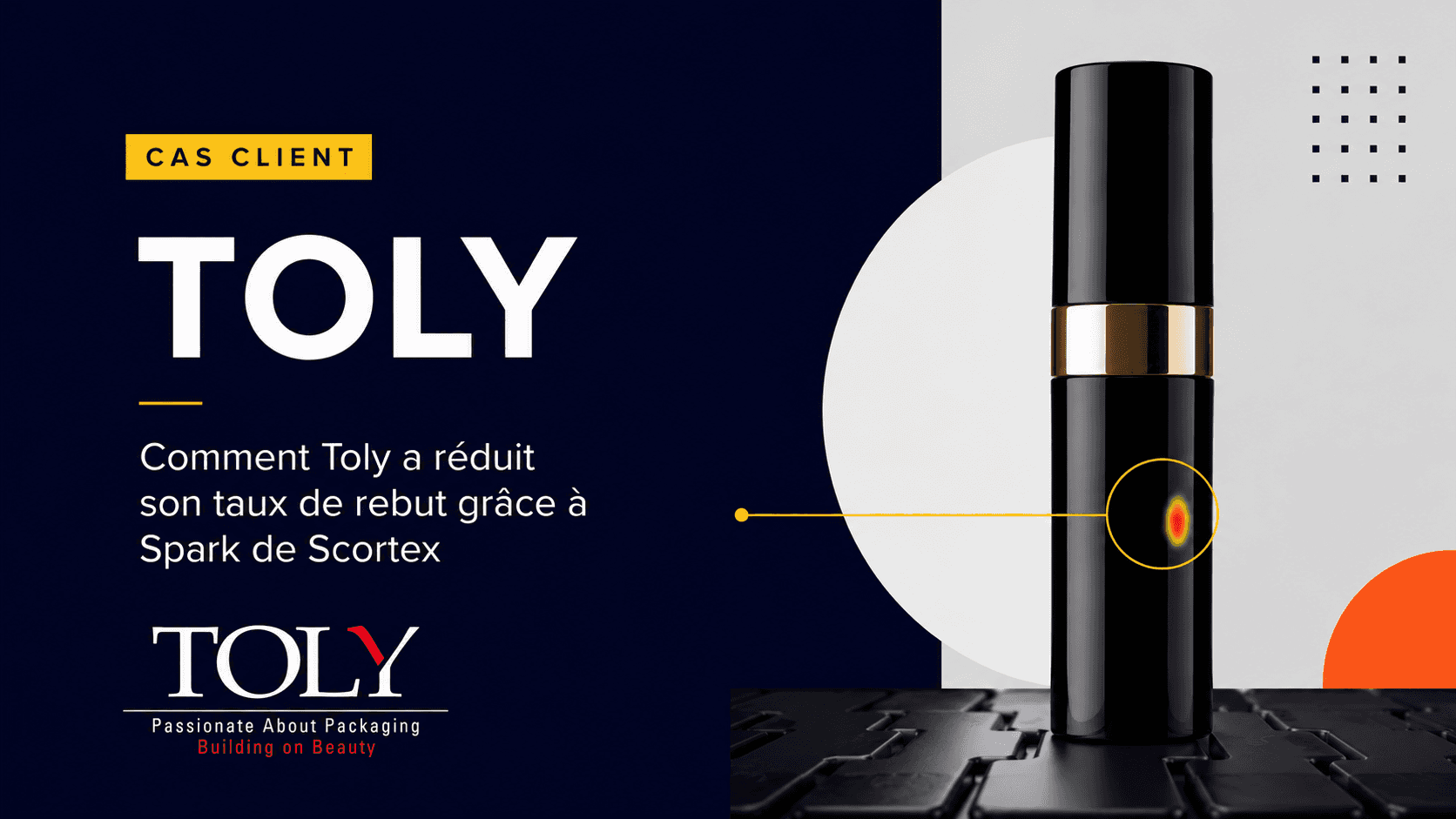
L'Automatisation du contrôle qualité chez Toly grâce à la technologie Spark de Scortex
L'équipe Scortex

La vision industrielle : qu'est-ce que c'est ?
L'équipe Scortex

7 missions clés d'un(e) Responsable Amélioration Continue pour un contrôle qualité optimal
L'équipe Scortex

Inspection qualité des pièces brillantes : un défi impossible à relever ?
L'équipe Scortex

Faut-il faire de la politique pour réussir un projet d’amélioration continue en qualité industrielle ?
L'équipe Scortex

Optimisation de la traçabilité suite au contrôle qualité dans l'industrie moderne : un pilier de la fiabilité et de la transparence
L'équipe Scortex

Rendre les spécifications qualité faciles à utiliser pour les opérateurs d'inspection - Etude de cas : Inspection sur ligne d’assemblage automobile
L'équipe Scortex

L'inspection qualité: pour quoi faire?
L'équipe Scortex

L'expérience utilisateur de votre solution de vision influence votre retour sur investissement
L’équipe Scortex

Conference EMVA X Scortex
L’équipe Scortex

Scortex x LVMH innovation awards & La Maison des Startups
L’équipe Scortex

Focus sur la qualité : votre plus grande opportunité d'améliorations opérationnelles et de réduction des coûts
L’équipe Scortex

Scortex - Partneraire technologique de COGNITWIN
L’équipe Scortex

Numérisation de l'inspection de la qualité pour l'industrie des plastiques
L’équipe Scortex

Numérisation de l'Inspection de Qualité pour l'Industrie de la Forge et de la Fonderie
L’équipe Scortex

Notre engagement en matière de sécurité
L’équipe Scortex

Une interview de Bill Black - Partie II
L’équipe Scortex
Une interview de Bill Black - Partie I
L’équipe Scortex

Scortex & SAP.IO Foundry Paris
L’équipe Scortex

Scortex au Mondial.Tech - Paris Motor Show 2018
L’équipe Scortex

Scortex sélectionné pour le programme Microsoft ScaleUp à Berlin.
L’équipe Scortex

Scortex remporte le Grand Prix au Concours "Startup Automobile".
L’équipe Scortex

Nous avons gagné le concours i-Lab
L’équipe Scortex

Annonce de notre Seed Funding
L’équipe Scortex

Sélectionné pour l'incubateur Agoranov
L’équipe Scortex
Tous
Education
Solution
News
Interviews
Comment Saverglass fiabilise l'inspection de ses bouteilles premium grâce à l'IA de Scortex
Equipe Scortex
Défauthèque industrielle : 8 erreurs à éviter lors de sa création
Equipe Scortex
Checklist défauthèque : les 15 points essentiels
Equipe Scortex
Créer une défauthèque industrielle : guide pratique
Equipe Scortex
Comment construire une défauthèque qualité efficace ?
Equipe Scortex
Comment identifier les défauts visuels critiques avant les réclamations client
Equipe Scortex
5 leviers pour améliorer l’analyse qualité
Equipe Scortex
Optimiser la performance qualité tout en réduisant rebuts et retouches
Equipe Scortex
Réduire les coûts cachés grâce au contrôle visuel automatisé
Comment structurer une défauthèque qualité pour sécuriser vos décisions
L'équipe Scortex
Protéger l’image des marques grâce au contrôle qualité des produits de luxe assisté par IA
L'équipe Scortex
Comment sécuriser le contrôle qualité des pièces métalliques avec l’IA
L'équipe Scortex
Automatiser le contrôle qualité des pièces en injection plastique par IA
L'équipe Scortex
Fiabiliser le contrôle qualité packaging avec un contrôle visuel automatisé
L'équipe Scortex
Comment sécuriser le contrôle qualité cosmétique grâce à l'automatisation
L'équipe Scortex
Contrôle qualité cosmétiques et packaging : fiabiliser l’inspection des surfaces exigeantes grâce à l’IA
Equipe Scortex
Contrôle qualité par l'IA : Scortex et IAR Group unissent leurs forces pour transformer le contrôle qualité industriel grâce à l'IA
L'équipe Scortex
7 missions clés d'un Responsable Qualité pour un contrôle qualité optimal
L'équipe Scortex
Comment aller au-delà des machines de tri qualité grâce à l'IA
L'équipe Scortex
Comment optimiser la qualité de production avec l'intelligence artificielle ?
L'équipe Scortex
Qu'est-ce que la traçabilité en contrôle qualité ? Explications simples
L'équipe Scortex
En quoi le contrôle qualité manuel et automatisé sont-ils complémentaires ?
L'équipe Scortex
Interview avec Hugues Poiget, CEO de Scortex
L'équipe Scortex
Dans les coulisses d'une marque de luxe qui a révolutionné le contrôle qualité de ses rouges à lèvres
L'équipe Scortex
Comprendre la norme qualité dans l'industrie automobile
L'équipe Scortex
5 façons de contrôler la qualité d'un produit
L'équipe Scortex
Défauthèque qualité : à quoi ça sert ?
L'équipe Scortex
Production cosmétique : défauts qualité visuels à éviter
L'équipe Scortex
Injection plastique : définition et fonctionnement
L'équipe Scortex
Les applications de l'intelligence artificielle en contrôle qualité
L'équipe Scortex
L'industrie 4.0, qu'est-ce que c'est ? Explications
L'équipe Scortex
Les avantages de l'inspection automatisée en contrôle qualité
L'équipe Scortex
L'Automatisation du contrôle qualité chez Toly grâce à la technologie Spark de Scortex
L'équipe Scortex
La vision industrielle : qu'est-ce que c'est ?
L'équipe Scortex
7 missions clés d'un(e) Responsable Amélioration Continue pour un contrôle qualité optimal
L'équipe Scortex
Inspection qualité des pièces brillantes : un défi impossible à relever ?
L'équipe Scortex
Faut-il faire de la politique pour réussir un projet d’amélioration continue en qualité industrielle ?
L'équipe Scortex
Optimisation de la traçabilité suite au contrôle qualité dans l'industrie moderne : un pilier de la fiabilité et de la transparence
L'équipe Scortex
Rendre les spécifications qualité faciles à utiliser pour les opérateurs d'inspection - Etude de cas : Inspection sur ligne d’assemblage automobile
L'équipe Scortex
L'inspection qualité: pour quoi faire?
L'équipe Scortex
L'expérience utilisateur de votre solution de vision influence votre retour sur investissement
L’équipe Scortex
Conference EMVA X Scortex
L’équipe Scortex
Scortex x LVMH innovation awards & La Maison des Startups
L’équipe Scortex
Focus sur la qualité : votre plus grande opportunité d'améliorations opérationnelles et de réduction des coûts
L’équipe Scortex
Scortex - Partneraire technologique de COGNITWIN
L’équipe Scortex
Numérisation de l'inspection de la qualité pour l'industrie des plastiques
L’équipe Scortex
Numérisation de l'Inspection de Qualité pour l'Industrie de la Forge et de la Fonderie
L’équipe Scortex
Notre engagement en matière de sécurité
L’équipe Scortex
Une interview de Bill Black - Partie II
L’équipe Scortex
Une interview de Bill Black - Partie I
L’équipe Scortex
Scortex & SAP.IO Foundry Paris
L’équipe Scortex
Scortex au Mondial.Tech - Paris Motor Show 2018
L’équipe Scortex
Scortex sélectionné pour le programme Microsoft ScaleUp à Berlin.
L’équipe Scortex
Scortex remporte le Grand Prix au Concours "Startup Automobile".
L’équipe Scortex
Nous avons gagné le concours i-Lab
L’équipe Scortex
Annonce de notre Seed Funding
L’équipe Scortex
Sélectionné pour l'incubateur Agoranov
L’équipe Scortex

Discutons de votre qualité dès aujourd'hui.

Les membres de l’équipe Scortex sont heureux de répondre à vos questions.
Discutons de votre qualité dès aujourd'hui.
Les membres de l’équipe Scortex sont heureux de répondre à vos questions.
Rejoignez notre newsletter
Rejoignez notre newsletter